
| 일 | 월 | 화 | 수 | 목 | 금 | 토 |
|---|---|---|---|---|---|---|
| 1 | 2 | 3 | ||||
| 4 | 5 | 6 | 7 | 8 | 9 | 10 |
| 11 | 12 | 13 | 14 | 15 | 16 | 17 |
| 18 | 19 | 20 | 21 | 22 | 23 | 24 |
| 25 | 26 | 27 | 28 | 29 | 30 | 31 |
- spark udf
- TensorFlow
- Retry
- login crawling
- BigQuery
- API Gateway
- Counterfactual Explanations
- youtube data
- UDF
- 공분산
- flask
- 상관관계
- 유튜브 API
- gather_nd
- integrated gradient
- GenericGBQException
- requests
- Airflow
- API
- airflow subdag
- grad-cam
- hadoop
- chatGPT
- correlation
- session 유지
- top_k
- XAI
- GCP
- subdag
- tensorflow text
- Today
- Total
데이터과학 삼학년
한개의 모델로 성격이 비슷한 여러개의 모델을 대체해보자 본문
다변량 시계열 분석을 위해 LSTM을 활용하고 있다. 다만, LSTM을 여러개의 모델을 구성해야 할때가 있다.
예를 들어 내가 분석하고자하는 서버가 20개 이면 20개 모델을 구해야하는데..
나는 서버 구분없이 모든 서버를 대표할 수 있는 일명 allround 용 모델 하나를 생성하고 싶다.
이를 위해 여러 방법을 시도해보았고, 그 중 잘 working한 모델을 공유하려 한다.
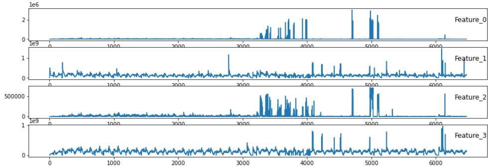
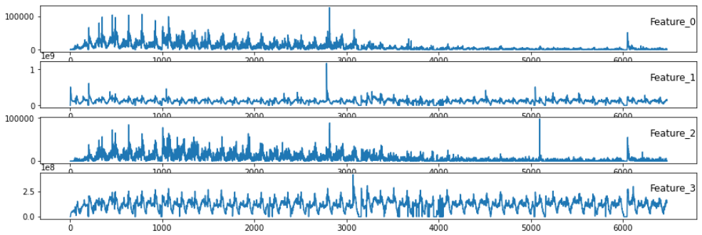
아래와 같이 서버별 시계열 데이터가 상이한 케이스가 있다.
1번 서버의 경우
2번 서버의 경우

위 그림과 같이 두개의 서버를 시계열 그래프로 나타내면 같은 FEATURE 라도 다른 양상을 보인다...
이럴경우, 각 서버별 모델을 구성해야한다는 것이다. 즉, 100개의 서버가 있으면 100개의 모델을 생성해서 분석해야한다.
이것은 정말 비용이 많이 드는 일이다..
이런 문제를 해결하기 위해 시간별 feature별 서버들의 중앙값을 가지고 모델을 학습해보았다.
이 가설은 결국 다변량 시계열 모델은 각 feature 별 어떠한 관계를 가지는지 기하학적으로 나타낼수 있을 것이고,
이 관계만 제대로 구할 수 있다면, 서버를 모두 커버할 수 있는 올라운드용 모델이 나오지 않을까란 생각에서다.
All Round 중앙값 모델 구하기
1. 중앙값을 이용한 시간별 데이터를 재구성 한다.
2. 위 데이터로 스케일링 후 예측하자
서버별 예측 결과
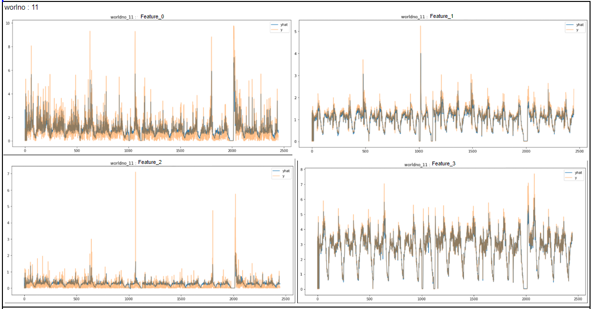
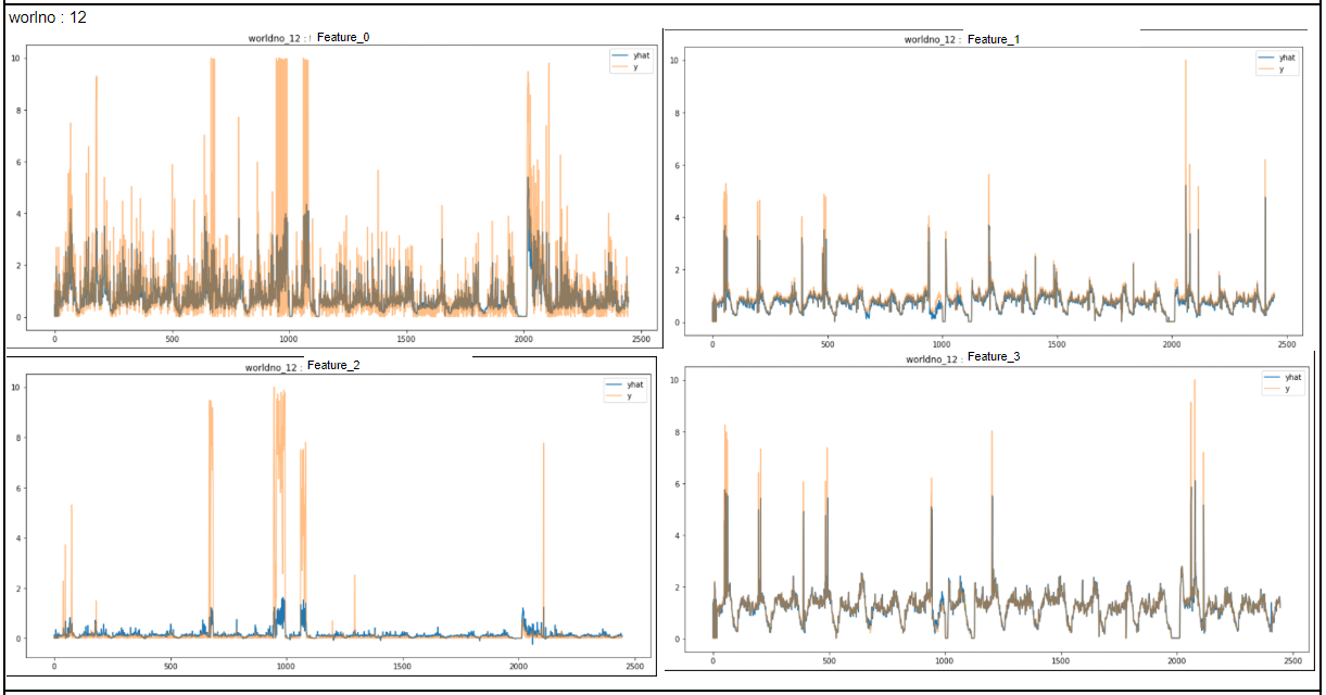
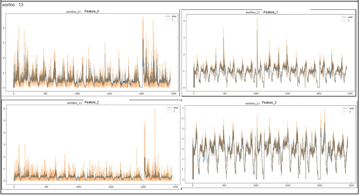
중앙값 모델을 가지고, 3개의 서버를 모두 대체할 만 한 결과를 얻었다!!!
아이디어를 내고, 그것을 실험한 끝에 얻을 수 있는 결과!!!
아주 간단한 아이디어였지만....
몇일을 어떻게 풀까 고민하며, 다른 알고리즘(VAR 등) 까지 고려하다 여기까지 왔다.
결국 머신러닝의 장점과 단점을 파악하고, 이것을 어떻게 쓸 지 고민하는 것!!!
이게 머신러닝 엔지니어의 역할이 아닌가 싶다.
도구는 사람이 어떻게 사용하냐에 따라 다르다는 것을 또 한번 느낀다...!
# prepare data for lstm
from pandas import read_csv
from pandas import DataFrame
from pandas import concat
from sklearn.preprocessing import LabelEncoder
from sklearn.preprocessing import MinMaxScaler, StandardScaler

# convert series to supervised learning
def series_to_supervised(data, n_in=1, n_out=1, dropnan=True):
	n_vars = 1 if type(data) is list else data.shape[1]
	df = DataFrame(data)
	cols, names = list(), list()
	# input sequence (t-n, ... t-1)
	for i in range(n_in, 0, -1):
		cols.append(df.shift(i))
		names += [('var%d(t-%d)' % (j+1, i)) for j in range(n_vars)]
	# forecast sequence (t, t+1, ... t+n)
	for i in range(0, n_out):
		cols.append(df.shift(-i))
		if i >= 0:
			names += [('var%d(t)' % (j+1)) for j in range(n_vars)]
# 		else:
# 			names += [('var%d(t+%d)' % (j+1, i)) for j in range(n_vars)]
	# put it all together
	agg = concat(cols, axis=1)
	agg.columns = names
	# drop rows with NaN values
	if dropnan:
		agg.dropna(inplace=True)
	return agg

    # load dataset
# dataset = read_csv('ts_data.csv', header=0, index_col=0)
values = ts_df.values
# integer encode direction
encoder = LabelEncoder()
values[:,0] = encoder.fit_transform(values[:,0])
# ensure all data is float
values = values.astype('float32')
# normalize features
scaler = MinMaxScaler(feature_range=(0, 10))
# scaler = StandardScaler()
scaled = scaler.fit_transform(values)
# frame as supervised learning
reframed = series_to_supervised(scaled, 1, 1)
# reframed = series_to_supervised(values, 1, 1)

# drop columns we don't want to predict
# reframed.drop(reframed.columns[[5,6,7]], axis=1, inplace=True)
print(reframed.head()) # 4개 변수로, get_ether 추정

reframed_r = reframed.reset_index()
reframed_r = reframed_r.drop(columns=['index'])
reframed_r

# split into train and test sets
values = reframed.values
n_train_hours = 24 * 6 * 28 # 4주
train = values[:n_train_hours, :]
test = values[n_train_hours:, :]
# split into input and outputs
train_X, train_y = train[:, :-4], train[:, -4:]
test_X, test_y = test[:, :-4], test[:, -4:]
# reshape input to be 3D [samples, timesteps, features]
train_X = train_X.reshape((train_X.shape[0], 1, train_X.shape[1]))
test_X = test_X.reshape((test_X.shape[0], 1, test_X.shape[1]))
print(train_X.shape, train_y.shape, test_X.shape, test_y.shape)

import tensorflow as tf
from tensorflow.keras.models import Sequential
from tensorflow.keras.layers import Dense
from tensorflow.keras.layers import LSTM
from tensorflow.keras import optimizers
# design network
learning_rate=0.001
model = Sequential()
model.add(LSTM(50, input_shape=(train_X.shape[1], train_X.shape[2])))
model.add(Dense(100))
model.add(Dense(4))
model.compile(optimizer=optimizers.Adam(learning_rate=learning_rate), loss='mae')
# fit network
history = model.fit(train_X, train_y, epochs=50, batch_size=32, validation_data=(test_X, test_y), verbose=2, shuffle=False)
# plot history
pyplot.plot(history.history['loss'], label='train')
pyplot.plot(history.history['val_loss'], label='test')
pyplot.legend()
pyplot.show()
### 중앙값 모델로 서버별 예측값 비교
df_11 = df[df.worldno==11]
df_12 = df[df.worldno==12]
df_13 = df[df.worldno==13]
def server_predict_plot(df,worldno):
ts_df = df[features]
values = ts_df.values
# integer encode direction
encoder = LabelEncoder()
values[:,0] = encoder.fit_transform(values[:,0])
# ensure all data is float
values = values.astype('float32')
# normalize features
scaler = MinMaxScaler(feature_range=(0, 10))
# scaler = StandardScaler()
scaled = scaler.fit_transform(values)
# frame as supervised learning
reframed = series_to_supervised(scaled, 1, 1)
# reframed = series_to_supervised(values, 1, 1)
# split into train and test sets
values = reframed.values
n_train_hours = 24 * 6 * 28 # 4주
test = values[n_train_hours:, :]
# split into input and outputs
test_X, test_y = test[:, :-4], test[:, -4:]
# reshape input to be 3D [samples, timesteps, features]
test_X = test_X.reshape((test_X.shape[0], 1, test_X.shape[1]))
yhat = model.predict(test_X)
from ipywidgets import interact
feature_dic = {ind:i for ind, i in enumerate(features)}
def compare_plot(feature_n):
pyplot.figure(figsize=(15,7))
pyplot.title('worldno_{} : '.format(worldno) + feature_dic[feature_n])
pyplot.plot(yhat[:,feature_n],label='yhat')
pyplot.plot(test_y[:,feature_n],alpha=0.5,label='y')
# pyplot.plot(resid,label='resid',alpha=0.3)
pyplot.legend()
interact(compare_plot,feature_n=[0,1,2,3])
server_predict_plot(df_11,11)
server_predict_plot(df_12,12)
server_predict_plot(df_13,13)'Machine Learning' 카테고리의 다른 글
| HDBSCAN vs DBSCAN (0) | 2021.07.08 |
|---|---|
| 배깅과 페이스팅 (Bagging, pasting) (2) | 2021.06.07 |
| Autoencoder 를 이용한 차원 축소 (latent representation) (0) | 2021.03.03 |
| PCA (Principal Component Analysis) 종류 (0) | 2021.02.02 |
| PCA (Principal Component Analysis) - 주성분 분석 (0) | 2021.01.13 |


